太疼的伤口，你不敢去触碰；太深的忧伤，你不敢去安慰；太残酷的残酷，有时候，你不敢去注视。 –龙应台 《目送》

In this session, we are going to focus on wide versus narrow dependencies, which dictate relationships between RDDs in graphs of computation, which we’ll see has a lot to do with shuffling.

So far, we have seen that some transformations significantly more expensive (latency) than others.

In this session we will:

• look at how RDD’s are represented
• dive into how and when Spark decides it must shuffle data
• see how these dependencies make fault tolerance possible

Lineages

Computations on RDDs are represented as a lineage graph, a DAG representing the computations done on the RDD. This representation/DAG is what Spark analyzes to do optimizations. Because of this, for a particular operation, it is possible to step back and figure out how a result of a computation is derived from a particular point.

1
2
3
4

val rdd = sc.textFile(...)
val filtered = rdd.map(...).filter(...).persist()
val count = filtered.count()
val reduced = filtered.reduce()

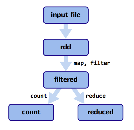
How RDDs are represented

RDDs are made up of 4 parts:

• Partitions: Atomic pieces of the dataset. One or many per compute node.
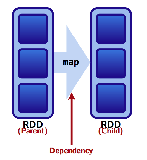
• Dependencies: Models relationship between this RDD and its partitions with the RDD(s) it was derived from. (Note that the dependencies maybe modeled per partition as shown below).
• A function for computing the dataset based on its parent RDDs.
• Metadata about it partitioning scheme and data placement.

/Users/caolei/IdeaProjects/untitled-life/source/images/post/.png

RDD Dependencies and Shuffles

Previously we saw the Rule of thumb: a shuffle can occur when the resulting RDD depends on other elements from the same RDD or another RDD.

In fact, RDD dependencies encode when data must move across network. Thus they tell us when data is going to be shuffled.

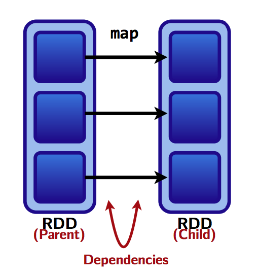
Transformations cause shuffles, and can have 2 kinds of dependencies: 1. Narrow dependencies: Each partition of the parent RDD is used by at most one partition of the child RDD.

1

[parent RDD partition] ---> [child RDD partition]

Fast! No shuffle necessary. Optimizations like pipelining possible. Thus transformations which have narrow dependencies are fast.

1. Wide dependencies: Each partition of the parent RDD may be used by multiple child partitions

1
2
3

                   ---> [child RDD partition 1]
[parent RDD partition] ---> [child RDD partition 2]
                   ---> [child RDD partition 3]

Slow! Shuffle necessary for all or some data over the network. Thus transformations which have narrow dependencies are slow.

Visual: Narrow dependencies Vs. Wide dependencies

Visual: Example

Assume that we have a following DAG:

What do the dependencies look like? Which are wide and which are narrow?

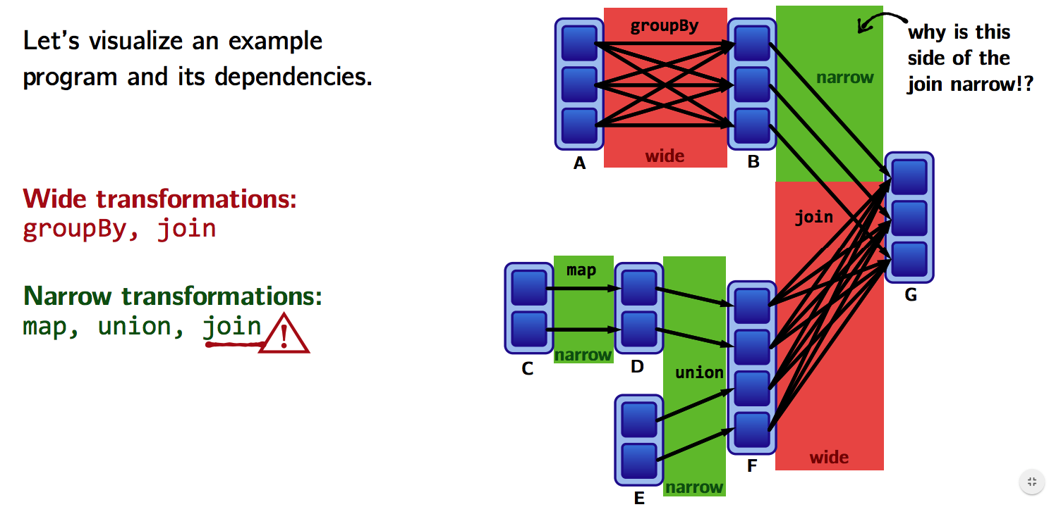
The B to G join is narrow because groupByKey already partitions the keys and places them appropriately in B after shuffling.

Thus operations like join can sometimes be narrow and sometimes be wide.

Transformations with (usually) Narrow dependencies: - map - mapValues - flatMap - filter - mapPartitions - mapPartitionsWithIndex

Transformations with (usually) Wide dependencies: (might cause a shuffle) - cogroup - groupWith - join - leftOuterJoin - rightOuterJoin - groupByKey - reduceByKey - combineByKey - distinct - intersection - repartition - coalesce

This list usually holds, but as seen above, in case of join, depending on the use case, the dependency of an operation may be different from the above lists

How can I find out?

dependencies method on RDDs: returns a sequence of Dependency objects, which are actually the dependencies used by Spark’s scheduler to know how this RDD depends on RDDs.

The sorts of dependency objects that this method may return include:

• Narrow dependency objects

  • OneToOneDependency
  • PruneDependency
  • RangeDependency

• Wide dependency objects

  • ShuffleDependency

Another method toDebugString prints out a visualization of the RDD lineage along with other information relevant to scheduling. For example, indentations in the output separate groups of narrow transformations that may be pipelined together with wide transformations that require shuffles. These groupings are called stages.

Example

1
2
3
4
5
6
7
8
9
10
11
12
13
14
15
16
17
18

val wordsRDD = sc.parallelize(largeList)

/* dependencies */

val pairs = wordsRdd.map(c=>(c,1))
                    .groupByKey
                    .dependencies          // <-------------
// pairs: Seq[org.apache.spark.Dependency[_]] = List(org.apache.spark.ShuffleDependency@4294a23d)

/* toDebugString */

val pairs = wordsRdd.map(c=>(c,1))
                    .groupByKey
                    .toDebugString         // <-------------
// pairs: String =
// (8) ShuffledRDD[219] at groupByKey at <console>:38 []
//  +-(8) MapPartitionsRDD[218] at map at <console>:37 []
//     | ParallelCollectionRDD[217] at parallelize at <console>:36 []

Lineages and Fault Tolerance

Lineages are the key to fault tolerance in Spark

Ideas from functional programming enable fault tolerance in Spark:

• RDDs are immutable
• We use higher-order-functions like map,flatMap,filter to do functional transformations on this immutable data
• A function for computing the dataset based on its parent RDDs also is part of an RDD’s representation.

We just need to keep the information required by these 3 properties.

Along with keeping track of the dependency information between partitions as well, these 3 properties allow us to: Recover from failures by recomputing lost partitions from lineage graphs, as it is easy to back track in a lineage graph.

Thus we get Fault Tolerance without having to write the RDDs/Data to the disk! The whole data can be re-derived using the above information.

Visual Example

Lets assume one of our partitions from our previous example fails:

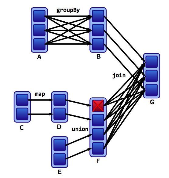
We only have to recompute the data shown below to get back on track:

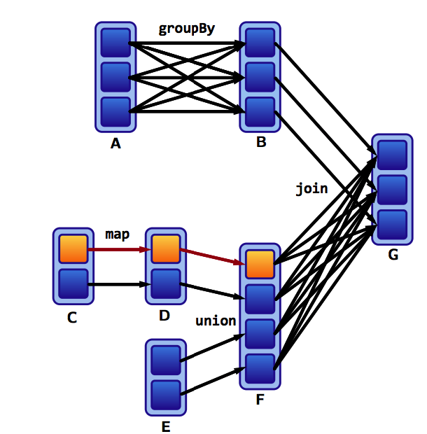
Recomputing missing partitions is fast for narrow but slow for wide dependencies. So if above, a partition in G would have failed, it would have taken us more time to recompute that partition. So losing partitions that were derived from a transformation with wide dependencies, can be much slower.

显示信息 http://untitled-life.github.io/blog/2018/12/27/wide-vs-narrow-dependencies/
written by Mike Cao  posted at http://untitled-life.github.io